RAG from Scratch (Part 1): Vectors, Embeddings and Vector Databases
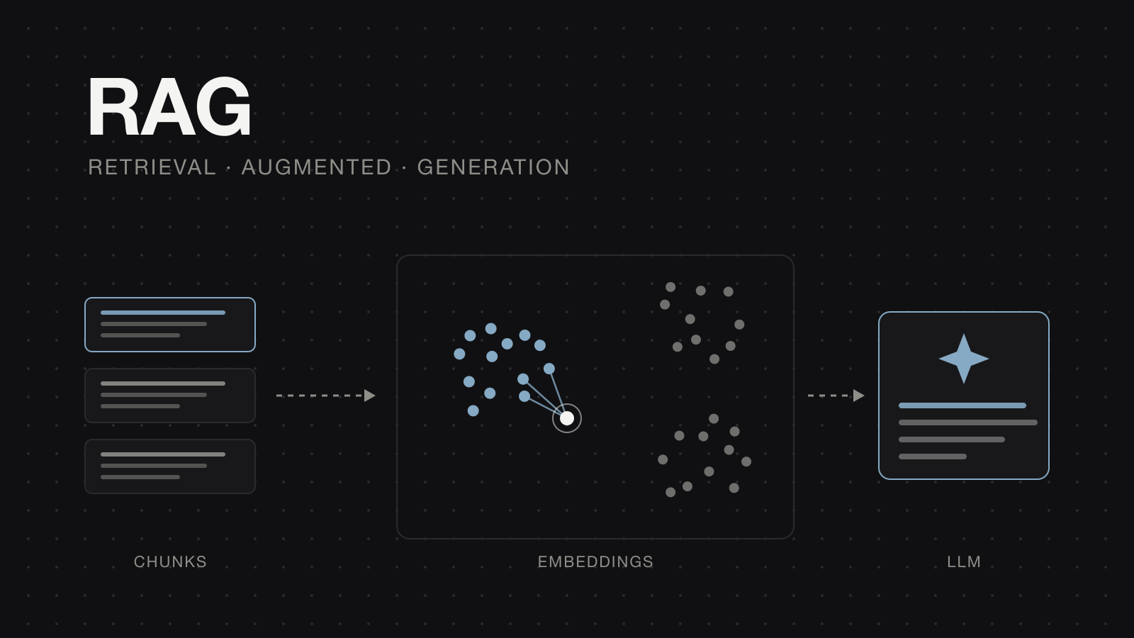
RAG (Retrieval-Augmented Generation) is one of the most widely used techniques for getting an LLM to answer with your own information —internal documents, manuals, policies— without retraining it. To really understand it you have to start with its building blocks: vectors, embeddings and vector databases. This article collects my notes on each of them, ordered from the most basic to the full picture.
This is part 1 of a series on RAG. Here we cover the fundamentals; in the next parts we’ll put them into practice.
What problem does RAG solve?
An LLM only knows what it saw during training. It knows nothing about your company’s internal documents or anything that changed after its cutoff date, and when it doesn’t know something it may make up an answer that sounds convincing.
RAG solves this in three steps that give it its name:
- Retrieval: finds the information relevant to the question in your own documents.
- Augmented: adds that information to the prompt as context.
- Generation: the LLM answers based on that context.
The key question is how to find “the relevant information” quickly and by meaning, not just by exact words. That’s what vectors, embeddings and a vector database are for.
Vectors: the foundation
A vector is an ordered list of numbers. Geometrically, you can picture it as an arrow with direction and magnitude:
- Direction tells you where it points.
- Magnitude is its length: how far it reaches in that direction.
In a three-dimensional space (x, y, z), the vector [3, 2, 1] points to a specific spot, and each axis is a dimension. The vectors used in AI work the same way, but with hundreds or thousands of dimensions:
[-0.12300456, 0.24304689, -0.15327687, 0.58767916, ...]Each number is the item’s position along one of those dimensions. What matters is that, in that space, the distance between two vectors can be measured, and that’s what will let us compare meanings.
Embeddings: vectors with meaning
An embedding is a vector that represents the meaning of a piece of content: a text, an image or an audio clip. It’s produced by an embedding model, a neural network trained so that content with similar meaning produces vectors that sit close together.
An embedding is a vector with meaning.
If we shrink the space down to just two dimensions, words with similar meanings end up clustered together:
quadrantChart
    title Simplified vector space (2 dimensions)
    x-axis "Animals" --> "Vehicles"
    y-axis "Small" --> "Large"
    Cat: [0.15, 0.25]
    Dog: [0.25, 0.35]
    Wolf: [0.3, 0.55]
    Bicycle: [0.7, 0.2]
    Car: [0.8, 0.5]
    Truck: [0.88, 0.82]
Cat and dog sit close together and far from truck. A real model does the same thing, just with hundreds of dimensions. One caveat: in this example each axis has a name (“animals”, “size”) to make it easy to read, but in a real model individual dimensions have no meaning of their own. Traits like topic, tone or context are spread across many of them at once.
The general path for turning data into embeddings looks like this:
flowchart LR
    A["Text · Image<br/>Audio · Video<br/><i>Unstructured data</i>"]
    B["Embedding model<br/><i>Turned into embeddings</i>"]
    C["[0.12, -0.48, …, 0.33]<br/>[0.91, 0.05, …, -0.27]<br/>[-0.36, 0.72, …, 0.14]<br/><i>Embeddings</i>"]
    D[("Vector database<br/><i>Storage</i>")]
    A -->|input| B -->|produces| C -->|stored in| D
Vector databases
A vector database stores embeddings and lets you find the ones closest to a given vector. Unlike a traditional search, which matches exact words, it searches by similarity of meaning: a query about “programming courses” can find a document about “software development training” even if they share no words at all.
Each record usually holds three things:
- The vector (embedding), used for searching.
- The chunk’s original text, which is what gets returned.
- Optional metadata, such as the source document or date, used for filtering.
For search to work, the database has to answer two questions: how to measure how alike two vectors are, and how to search quickly among millions of them.
flowchart TD
    BD[("Vector database")]
    BD --> SIM["Similarity measures<br/><i>how alike are they?</i>"]
    BD --> IDX["Search and indexing<br/><i>how to find them fast?</i>"]
    SIM --> COS["Cosine<br/><i>compares the angle</i>"]
    SIM --> L2["L2 distance<br/><i>measures distance</i>"]
    SIM --> DOT["Dot product<br/><i>angle + magnitude</i>"]
    IDX --> KNN["Exact KNN<br/><i>compares against all:<br/>accurate, but slow</i>"]
    IDX --> ANN["Approximate ANN<br/><i>indexes like HNSW or IVF:<br/>prioritizes speed</i>"]
Similarity measures
They let you quantify how alike two vectors are:
- Cosine similarity: compares the angle between vectors, that is, only their direction. It’s the most common choice for text embeddings. The higher the value, the more alike.
- L2 distance (L2 norm or Euclidean distance): measures the straight-line distance between the two points. The smaller the distance, the more alike.
- Dot product: combines direction and magnitude. If the vectors are normalized (all with magnitude 1), it ranks results the same way as cosine similarity.
The safest choice is the measure the embedding model was trained for; its documentation usually says which one.
Search and indexing
Finding the vectors closest to a query is known as nearest neighbor search. There are two approaches:
- Exact KNN (k-nearest neighbors): compares the query against every stored vector. It always finds the closest ones, but gets slow once you have millions of records.
- ANN (approximate nearest neighbors): uses an index that organizes the vectors ahead of time —for example HNSW, graph-based, or IVF, cluster-based— so only part of them needs checking. It trades a bit of accuracy for a lot of speed, and it’s what most production vector databases use.
Ingestion: how information gets loaded
Before you can search, the documents have to be loaded into the vector database. This process is called ingestion and it runs once, or whenever the documents change:
flowchart LR
    A["<b>1. Raw data</b><br/>Text<br/>Image / video<br/>Documents"]
    B["<b>2. Preprocessing</b><br/>Cleans what adds nothing:<br/>line breaks, spaces,<br/>special characters"]
    C["<b>3. Chunking</b><br/>Splits into fragments<br/>(chunks)"]
    D["<b>4. Embedding model</b><br/>Turns each chunk<br/>into a vector"]
    E[("<b>5. Storage</b><br/>Vector + text<br/>+ metadata")]
    A --> B --> C --> D --> E
- Raw data: text, images, videos or documents such as PDFs.
- Preprocessing: strips whatever carries no meaning, such as line breaks, repeated spaces or special characters. What to clean depends on the case: emojis, for example, can be noise or can convey the tone of a message.
- Chunking: the document is split into smaller fragments.
- Embedding model: each chunk is turned into a vector.
- Storage: each vector is saved along with its text and metadata.
Why split into chunks?
A large document isn’t turned into a single vector, for two reasons. Embedding models have a limit on how much text they can process, and a vector summarizing fifty pages mixes too many topics to be found precisely. With chunks, each vector represents one concrete idea:
flowchart LR
    PDF["📄 PDF<br/><i>Document</i>"]
    subgraph S["Chunking"]
        C1[chunk]
        C2[chunk]
        C3[chunk]
    end
    subgraph M["Embedding model"]
        E1[embed]
        E2[embed]
        E3[embed]
    end
    subgraph DB["Vector database"]
        V1["[0.51, 0.30, 0.51]<br/><i>+ chunk text</i>"]
        V2["[0.43, 0.32, 0.37]<br/><i>+ chunk text</i>"]
        V3["[0.12, 0.47, 0.28]<br/><i>+ chunk text</i>"]
    end
    PDF --> C1 --> E1 --> V1
    PDF --> C2 --> E2 --> V2
    PDF --> C3 --> E3 --> V3
Each chunk produces one vector, and the database stores that vector alongside the original text. That detail matters: search compares vectors, but what gets retrieved and handed to the LLM is the text.
The three-number vectors in these examples are a simplification. A real embedding has hundreds or thousands of dimensions.
Querying: how a question gets answered
Once the information is loaded, this is how a question gets answered:
sequenceDiagram
    actor U as User
    participant App as RAG application
    participant E as Embedding model
    participant DB as Vector database
    participant L as LLM
    U->>App: 1. "I want a programming course"
    App->>E: 2. Converts the query
    E-->>App: [0.54, 0.32, 0.12]
    App->>DB: 3. Searches for the closest vectors
    Note over DB: Compares using a similarity<br/>measure (e.g. cosine)
    DB-->>App: 4. The k most similar chunks
    App->>L: 5. Prompt = question + chunks as context
    L-->>App: Generated answer
    App->>U: 6. Answer to the user
- The user asks something, for example: “I want a programming course”.
- The query is turned into an embedding with the same model used during ingestion:
[0.54, 0.32, 0.12]. With different models, the vectors wouldn’t be comparable. - The vector database compares the query vector with the stored ones, using the configured similarity measure.
- The k most similar chunks (the top-k, usually between 3 and 10) are retrieved along with their text. For example, the chunk whose vector is
[0.51, 0.30, 0.51]. - The LLM receives the question along with those chunks as context and generates an answer based on them.
- The answer reaches the user.
The full RAG model
Putting all the pieces together, this is the path a query takes through the three RAG stages:
flowchart TB
    U(["👤 User"]) -->|question| Q[Query]
    subgraph R["1 · Retrieval"]
        EMQ["Embedding model<br/><i>same one used at ingestion</i>"] -->|query vector| DB[("Vector database<br/><i>loaded at ingestion</i>")]
    end
    subgraph A["2 · Augmented · context enrichment"]
        CTX[Context] --> PT["Prompt template<br/><i>instructions + context + question</i>"]
    end
    subgraph G["3 · Generation · answer generation"]
        LLM[LLM]
    end
    Q --> EMQ
    Q -->|original question| PT
    DB -->|most similar chunks| CTX
    PT -->|enriched prompt| LLM
    LLM --> ANS(["👤 Answer to the user"])
- Retrieval: the query is turned into an embedding and the most similar chunks are looked up in the vector database.
- Augmented (context enrichment): those chunks are inserted into a prompt template, along with instructions (for example, “answer only with the information in the context”) and the original question.
- Generation: the LLM answers based on that enriched context.
Ingestion happens only once; these three stages run on every query.
Conclusion
RAG isn’t magic: it’s a vector database that finds the content whose meaning is closest to the question, and an LLM that writes the answer using that content as context. Understanding vectors and embeddings is what lets you make good decisions when implementing it: how to chunk your documents, which embedding model to use, which similarity measure to choose and how many chunks to retrieve.
In part 2 of this series we’ll walk through a technical example to see all of these concepts in action.